
algebra
Types of matrices

Matrices are fundamental concepts in mathematics, physics, computer science, and engineering. Let us explore more various forms of matrices and their unique characteristics. Here are some different types of matrices with examples.
1. Periodic Matrix: A periodic matrix is a square matrix. A that meets the requirements.
![]()
Example:
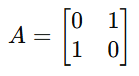
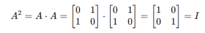
Thus A^2=I and the period of A is k=2.
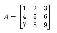
2. Real Matrix: A real matrix has entries (elements) that are all real numbers. A real matrix is a rectangular array whose elements are all real integers (R).
Example:
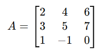
Here, A is a 3×3 real matrix because all its entries are real numbers.
3.Imaginary Matrix: An imaginary matrix is a matrix in which all the elements are purely imaginary numbers. A purely imaginary number is of the form bi, where (a real number) and ii is the imaginary unit . (i=![]() )
)
Example:
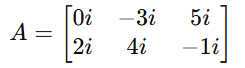
Here, All the entries are purely imaginary numbers like 0i, -3i, 5i etc.
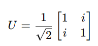
4. Unitary matrix: A unitary matrix is a complex square matrix U that meets the following condition:
![]()
Where,
 is the conjugate transpose of U ( transpose of the matrix after obtaining the complex conjugate of each member).
- is the identity matrix of the same dimension.
Example:
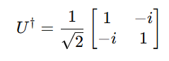
Compute the conjugate transpose.
Verify the Unitary property
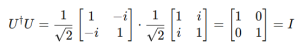
Thus,U is a unitary matrix.
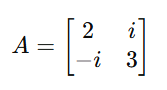
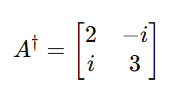
5. Normal Matrix: A normal matrix is a square matrix that commutes with its conjugate transpose, meaning:
![]()
Where,
 is the conjugate transpose of A ( transpose of A with the complex conjugate each element )
- is defined over the field of complex numbers but can also be real.
Example:
Conjugate transpose:
Verify ![]()
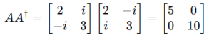
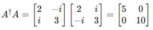
Thus, A is a normal matrix.
6. Hermitian Matrix: A Hermitian matrix is a square matrix that equals its own conjugate transpose. In other words, a matrix A is Hermitian if:
![]()
where A^H is the conjugate transpose of . This means that the element in the -th row and j-th column is the complex conjugate of the element in the j-th row and i-th column. Mathematically:
![]()
Example:
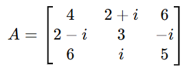
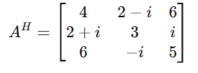
Here,
- The diagonal elements 4, 3, 5 are real.
- A12=2+i ,A21=2-i, showing the required conjugate symmetry.
- A13=6, A31=6 as 6 is its own conjugate.
- A23=-i,A32=i
Since ![]() , the matrix A is Hermitian.
, the matrix A is Hermitian.
7.Skew Hermitian: A skew-Hermitian matrix is a square matrix 𝐴 that meets the following condition:
![]()
Here, A^H is the conjugate transpose of . This means the element in the -th row and -th column is the negative complex conjugate of the element in the -th row and -th column. Mathematically:
![]()
Example:
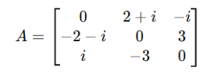
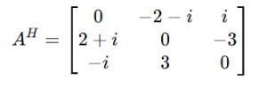
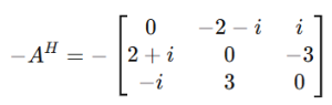
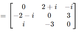
Here,
- The diagonal elements (0, 0, 0) are purely imaginary or zero.
- A12= 2+i, A21=-2-i
- A13=-i, A31=i
Since,![]() the matrix A is skew hermitian.
the matrix A is skew hermitian.
8. Sub Matrix: A submatrix is a smaller matrix that is formed by selecting certain rows and/or columns from a larger matrix while maintaining their order.
How to create sub matrix
- Start with a given matrix
- Select particular rows and columns to add to the submatrix.
- Remove the unwanted rows and/or columns.
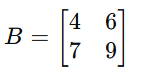
Example 1 : Submatrix from a 3×3 Matrix
Submatrix by Removing the 1st Row and 2nd Column:
- Remove the 1st row: {1, 2, 3}
- Remove the 2nd column: {2, 5, 8}
The submatrix is:
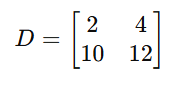
Example 2: Submatrix from a 4×4 Matrix
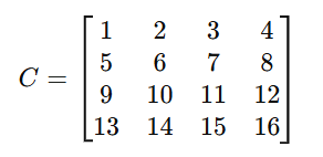
Submatrix by Keeping the 1st, 3rd Rows and 2nd, 4th Columns:
- Keep rows {1,3}: {1,2,3,4} and {9,10,11,12}
- Keep columns {2,4}: {2,4} and {10,12}
The submatrix is:
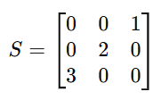
9. Sparse Matrix: A Sparse Matrix has a majority of its elements as zero.
Example:
Each Types of matrices serves a unique purpose, from simplifying computations to modeling real-world problems. We have to know all Different Types of matrices for tackling challenges in mathematics, science, and technology.

The Gauss-Jordan elimination example is an algorithm used to solve systems of linear equations. It transforms the argumented matrix of the system into its reduced row echelon form (RREF) , allowing for the direct reading of solutions .Here’s a step-by-step explanation:
Steps in Gauss-Jordan Elimination
- From the argumented matrix: Create an augmented matrix by combining the equations’ constants and variable coefficients.
- Make the leading coefficient (pivot) of the first row equal to 1:
- Divide the first row by its pivot (the first non-zero element).
- This ensures the pivot becomes 1.
3. Eliminate all other entries in the pivot column:
- Use row operations to make all elements below and above the pivot equal to 0
4. Move to the next pivot:
- To locate the pivot, which is usually the diagonal element, choose the following row and column.
- Repeat steps 2 and 3 to make this pivot 1 and elliminate other entries in its column.
5. Continue until the matrix is in reduced row echelon form (rref):
- A matrix is in RREF if:
- Each leading entry in a row is 1.
- Each leading 1 represents the lone non-zero value in its column.
- Rows with only zeros are at the bottom.
6. Read the Solution:
- The final column of the augmented matrix gives the solution to the system.
Gauss-Jordan elimination example
Solve the system of equations

1. From the argumented matrix :

2. Perform row operations:
Step 1: Make the pivot at (1,1) equal to 1
Divide row 1 by 2

Step 2: Eliminate elements below the pivot (1,1)
- Add 3×Row 1 to Row 2
- Add 2× to Row 3.
Result:

Step 3: Make the pivot at (2,2) equal to 1.
Divide Row 2 by 0.5:

Step 4: Eliminate elements below and above the pivot (2,2).
- Subtract 2×Row2 from Row 3.
- Subtract 0.5×Row 2 from Row 1.
Result

Step 5 : Make the pivot at (3,3) equal to 1
Divide row 3 by -1

Step 6: Eliminate elements above the pivot (3,3)
- To Row 1, add Row 3.
- Take Row 2 and subtract Row 3.
Result:

3. Read the solution
From the final matrix
![]()


Cramer’s rule 2×2 , 3×3 is a method used to solve systems of linear equations using determinants. So It applies to systems of n linear equations with n variables, assuming that the determinent of the co-efficient matrix is non zero. This rule provides precise formulas for solving a system of linear equations using determinants.
Consider this system of linear equations:
![]()
where:
- A is a square matrix (with size n×n)
- x is a column vector of unknowns x_1,x_2,…,x_ n,
- b represents a column vector of constants. b_1,b_2,…,b_n
The matrix equation can be written as:

Step-by-Step Instructions for Cramer’s rule 2×2
1. Calculate the determinant of the coefficient matrix: Check if matrix A’s determinant (det(𝐴)) is non-zero. Because if det(A) = 0, the system lacks a unique solution and cannot be solved using Cramer’s Rule.
2. Construct Matrices A_1, A_2,…, A_n: For each unknown x_i, construct a new matrix A_i by substituting the i-th column of matrix A with the column vector b. Substitute the constants from vector b for the i-th column of A to produce the i-th matrix A_i.
- is formed by replacing the first column of A with b
- A2 is created by substituting b for A’s second column.
- and so on for all columns.
3. Calculate the determinants of the modified matrix: Determine the determinant of each matrix A i, denoted as det(A_i), for each i=1, 2,…,n.
4. Solve for Each x_i: The solution for each unknown x_i is given by:

for i=1,2,…,n.
For example:
Consider this system of linear equations:

The coefficient matrix is:

The column vector b is

Step 1: Firstly, Calculate det(A)
![]()
Step 2: Create matrices A_1 and A_2.
- For x, replace the first column of A with b:

- For y, change the second column of A to b:

Step 3: Compute the determinants of A_1 and A_2
![]()
![]()
then,
Step 4: Solve for x and y:


So, lastly, the solution to the system is:

Cramer’s rule 2×2 simplifies the process of solving linear equations using determinants. However, it is computationally expensive for big systems due to the necessity to calculate numerous determinants.
Practice problems
1.

2.

3.

4.


All formulas of circle-Concepts , Properties

How to make math fun through storytelling: Chapter 3

Types of progression (AP,GP,HP progression)

Fun math learning stories: The secret of the shadow pyramid

Math problem-solving stories: The Secret of the Shadow Pyramid

Vector properties (Definition, Examples)

Three-dimensional coordinate geometry: Formulas ,Examples

Educational math stories : Chapter 5: The infinity Chamber

Algebra puzzles and riddles for children: Chapter 4- Labyrinth of patterns

How can I make algebra fun for kids? Chapter 3- Tower of Variables


Fun math learning stories: The secret of the shadow pyramid
Math problem-solving stories: The Secret of the Shadow Pyramid
Vector properties (Definition, Examples)
Three-dimensional coordinate geometry: Formulas ,Examples
Educational math stories : Chapter 5: The infinity Chamber
Algebra puzzles and riddles for children: Chapter 4- Labyrinth of patterns
-
 algebra3 months ago
Various types of matrices
-
 algebra3 months ago
Trigonometric Rules and Formulas
-

 geometry3 months ago
Cartesian to polar equations (Circle, line)
-

 algebra3 months ago
Cayley-Hamilton theorem matrix
-

 algebra3 months ago
Eigenvalue of a matrix
-

 algebra4 months ago
Different types of Matrices
-

 calculus4 months ago
Easy Strategies & Techniques for Effective Integration part-1
-
 geometry3 months ago
Cartesian coordinate planes (Polar to cartesian)