
algebra
Echelon Row Reduction

An echelon matrix is a matrix that has been transformed to a specific structured form using row operations. The most common types are row echelon form (REF) and reduced row echelon form (RREF). The Echelon Row Reduction process is widely used in solving systems of linear equations, performing Gaussian elimination, and analyzing linear algebra properties. Here is an example of echelon row reduction.
Row Echelon Form (REF)
A matrix is in reduced row echelon form if:
- The zero rows (if any) are at the bottom of the matrix.
- The leading (first non-zero) entry in each non-zero row is to the right of the preceding row’s leading entry.
- Every entry that comes after a leading entry is zero.
Example:
Reduced Row Echelon Form (RREF)
A matrix is in reduced row echelon form if:
- It meets every requirement of the row echelon form.
- Every non-zero row has a leading entry of 1 (called a leading 1).
- Each leading 1 represents the only non-zero value in its column.
Example:
Here’s an example of converting a matrix into Row Echelon Form (REF) and Reduced Row Echelon Form (RREF) using Gaussian and Gauss-Jordan elimination, respectively.
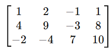
Problem:
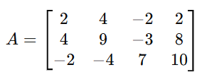
Step1: Transform to row echelon form
To add zeros below the pivot places, use row operations.
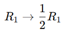
1. Divide the first row by 2 (make the leading entry 1):
2. Eliminate the first column entries below the pivot (1 in R1[1,1])
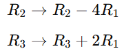
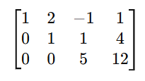
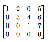
Now, the matrix is in Row Echelon Form (REF).
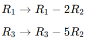
Step 2: Transform to Reduced Row Echelon Form (RREF)
Use row operations to set the pivot entries to 1 and remove any non-zero items from the pivot columns.
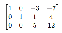
1. Make the pivot in the second row 1 (already done) and eliminate the second column entries above and below it:
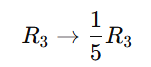
2. Make the pivot in the third row 1 by dividing R3 by 5:
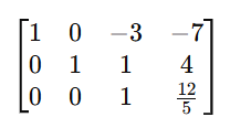
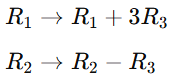
3. Remove the third column entries above the pivot in R 3 [3, 3].
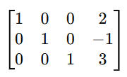
Now, the matrix is in Reduced Row Echelon Form (RREF).
Final forms:
Row Echelon Form (REF):
Reduced Row Echelon Form (RREF):

The Gauss-Jordan elimination example is an algorithm used to solve systems of linear equations. It transforms the argumented matrix of the system into its reduced row echelon form (RREF) , allowing for the direct reading of solutions .Here’s a step-by-step explanation:
Steps in Gauss-Jordan Elimination
- From the argumented matrix: Create an augmented matrix by combining the equations’ constants and variable coefficients.
- Make the leading coefficient (pivot) of the first row equal to 1:
- Divide the first row by its pivot (the first non-zero element).
- This ensures the pivot becomes 1.
3. Eliminate all other entries in the pivot column:
- Use row operations to make all elements below and above the pivot equal to 0
4. Move to the next pivot:
- To locate the pivot, which is usually the diagonal element, choose the following row and column.
- Repeat steps 2 and 3 to make this pivot 1 and elliminate other entries in its column.
5. Continue until the matrix is in reduced row echelon form (rref):
- A matrix is in RREF if:
- Each leading entry in a row is 1.
- Each leading 1 represents the lone non-zero value in its column.
- Rows with only zeros are at the bottom.

6. Read the Solution:
- The final column of the augmented matrix gives the solution to the system.
Gauss-Jordan elimination example
Solve the system of equations

1. From the argumented matrix :

2. Perform row operations:
Step 1: Make the pivot at (1,1) equal to 1
Divide row 1 by 2

Step 2: Eliminate elements below the pivot (1,1)
- Add 3×Row 1 to Row 2
- Add 2× to Row 3.
Result:

Step 3: Make the pivot at (2,2) equal to 1.
Divide Row 2 by 0.5:

Step 4: Eliminate elements below and above the pivot (2,2).
- Subtract 2×Row2 from Row 3.
- Subtract 0.5×Row 2 from Row 1.
Result

Step 5 : Make the pivot at (3,3) equal to 1
Divide row 3 by -1

Step 6: Eliminate elements above the pivot (3,3)
- To Row 1, add Row 3.
- Take Row 2 and subtract Row 3.
Result:

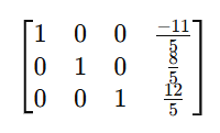
3. Read the solution
From the final matrix
![]()

Definition of vector space
Subspace and vector space : A vector space V over a field F (typically R or C) consists of:
- A set of elements known as vectors.
- Scalars are a set of elements from a field (𝐹).
The following operations have been defined:
Vector addition: + : V×V→V, where u+v is the sum of u and v in V.
Scalar multiplication: ⋅ : F×V→V, where a⋅v is the scalar multiplication of a∈F with v∈V.
Axioms of a vector space
The following must be true for any scalars a,b∈F and vectors u,v,w∈V:
1. Addition Properties:
- Associativity: u+(v+w)=(u+v)+w.
- Commutativity: u+v=v+u.
- The identity element of addition: There exists a vector 0 ∈ V such that u + 0 = u for all u∈V.
- Inverse elements of addition: For every u∈V, there exists −u∈V such that u+(−u)=0 .
2. Scalar multiplication properties:
- Distributivity with respect to vector addition: a⋅(u+v)=a⋅u+a⋅v
- Distributivity with respect to scalar addition: (a+b)⋅v=a⋅v+b⋅v
- Compatibility of Scalar Multiplication: (a⋅b)⋅v=a⋅(b⋅v)
- identity element of Scalar multiplication: 1⋅v=v, where 1 is the multiplicative identity in F.
Examples of Vector Space
1. Real coordinate space R^n:
- Vectors: ordered tuples (x_1, x _2, …, x_ n ) with x_i ∈ R
- Scalar: real numbers R.
2. Complex coordinate space ( C^n):
- Vectors: ordered tuples (z_1,z_2,…,z_ n) with z_i∈C.
- Scalar: complex numbers C.
3. Function space:
- Vectors : functions f:X→R (or C)
- Scalar: real or complex numbers
4. Polynomials:
- Vectors : Polynomials p(x)=a_0 +a_1 x+⋯+a_n x^ n
- Scalar: coefficients 𝑎_𝑖∈F from the field F .

Subspace
A subspace is a subset of a vector space that is also a vector space, subject to the same scalar multiplication and vector addition operations. Stated otherwise, if V is a vector space, then a subspace of V is a subset W⊆V that satisfies vector space requirements by applying the same operations described in V.
Condition for Subspaces
Assume V is a vector space over a field F, and W is a subset of V. To be a subspace of V, W must meet the following conditions:
- Zero Vector: The zero vector of must be in , i.e., 0∈W
- Closed under Addition: Any two vectors u,v∈W, their sum must also be in W, i.e., u+v ∈ W.
- Closed under Scalar Multiplication: For any vector u∈W and scalar a∈F, the scalar multiple a⋅u must also be in , i.e., a⋅u∈W.
These three requirements are necessary for W to be a subspace. Importantly, the vector space axioms of V already guarantee other qualities, such as associativity, commutativity, etc., so we don’t need to verify them. Additionally, keep in mind that W will inherit every other property of a vector space if these requirements are met.
Key properties of subspace
- A subspace always contains the zero vector of the original vector space.
- Subspaces are closed under addition and scalar multiplication.
- The intersection of two subspaces is always a subspace.
- The span of any subset of a vector space is a subspace. (The span is the set of all linear combinations of the subset’s elements.)
Examples of subspaces
1. Subspace of R^3:
- Consider the vector space R^3 , the set of all 3-dimensional vectors with real coordinates.
- A plane passing through the origin (such as the xy plane) is a subspace of R^3. This is because it contains the zero vector, is closed under vector addition, and is closed under scalar multiplication.
2. The set of all polynomials of degree less than or equal to n:
- The set of all polynomials of degree less than or equal to n is a subspace of the vector space of all polynomials . It is closed under addition and scalar multiplication.
3. The set of all solutions to a homogeneous linear system:
- A subspace of the vector space of all possible solutions is the set of all solutions to a system of linear equations (where the system is homogeneous, meaning the right-hand side is zero).
Non-Examples of subspaces
- A set without the zero vector: A set that does not contain the zero vector cannot be a subspace . For example , the set of all non zero vectors in R ^2 is not a subspace because it does not contain the zero vector.
- A Set Not Closed Under Addition or Scalar Multiplication : A set is not a subspace if it is not closed under scalar multiplication or addition. The set W={(x,y)∈R^2:x≥0}, for instance, is not a subspace since it is not closed under scalar multiplication (the outcome of multiplying a vector with a negative scalar may yield a vector that is not in W).

Cramer’s rule 2×2 , 3×3 is a method used to solve systems of linear equations using determinants. So It applies to systems of n linear equations with n variables, assuming that the determinent of the co-efficient matrix is non zero. This rule provides precise formulas for solving a system of linear equations using determinants.
Consider this system of linear equations:
![]()
where:
- A is a square matrix (with size n×n)
- x is a column vector of unknowns x_1,x_2,…,x_ n,
- b represents a column vector of constants. b_1,b_2,…,b_n
The matrix equation can be written as:

Step-by-Step Instructions for Cramer’s rule 2×2
1. Calculate the determinant of the coefficient matrix: Check if matrix A’s determinant (det(𝐴)) is non-zero. Because if det(A) = 0, the system lacks a unique solution and cannot be solved using Cramer’s Rule.
2. Construct Matrices A_1, A_2,…, A_n: For each unknown x_i, construct a new matrix A_i by substituting the i-th column of matrix A with the column vector b. Substitute the constants from vector b for the i-th column of A to produce the i-th matrix A_i.
- is formed by replacing the first column of A with b
- A2 is created by substituting b for A’s second column.
- and so on for all columns.
3. Calculate the determinants of the modified matrix: Determine the determinant of each matrix A i, denoted as det(A_i), for each i=1, 2,…,n.
4. Solve for Each x_i: The solution for each unknown x_i is given by:

for i=1,2,…,n.
For example:
Consider this system of linear equations:

The coefficient matrix is:

The column vector b is

Step 1: Firstly, Calculate det(A)
![]()
Step 2: Create matrices A_1 and A_2.
- For x, replace the first column of A with b:

- For y, change the second column of A to b:

Step 3: Compute the determinants of A_1 and A_2
![]()
![]()
then,
Step 4: Solve for x and y:


So, lastly, the solution to the system is:

Cramer’s rule 2×2 simplifies the process of solving linear equations using determinants. However, it is computationally expensive for big systems due to the necessity to calculate numerous determinants.
Practice problems
1.

2.

3.

4.


All formulas of circle-Concepts , Properties

How to make math fun through storytelling: Chapter 3

Types of progression (AP,GP,HP progression)

Fun math learning stories: The secret of the shadow pyramid

Math problem-solving stories: The Secret of the Shadow Pyramid

Vector properties (Definition, Examples)

Three-dimensional coordinate geometry: Formulas ,Examples

Educational math stories : Chapter 5: The infinity Chamber

Algebra puzzles and riddles for children: Chapter 4- Labyrinth of patterns

How can I make algebra fun for kids? Chapter 3- Tower of Variables


Fun math learning stories: The secret of the shadow pyramid
Math problem-solving stories: The Secret of the Shadow Pyramid
Vector properties (Definition, Examples)
Three-dimensional coordinate geometry: Formulas ,Examples
Educational math stories : Chapter 5: The infinity Chamber
Algebra puzzles and riddles for children: Chapter 4- Labyrinth of patterns
-
 algebra4 months ago
Various types of matrices
-
 algebra4 months ago
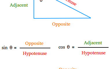
Trigonometric Rules and Formulas
-

 geometry4 months ago
Cartesian to polar equations (Circle, line)
-

 algebra5 months ago
Different types of Matrices
-

 algebra4 months ago
Cayley-Hamilton theorem matrix
-

 algebra5 months ago
Eigenvalue of a matrix
-

 calculus5 months ago
Easy Strategies & Techniques for Effective Integration part-1
-
 geometry3 months ago
Three-dimensional coordinate geometry: Formulas ,Examples