Cayley-Hamilton theorem matrix

A key concept of linear algebra is the Cayley-Hamilton theorem matrix, which states that each square matrix satisfies its own characteristic equation.

The Theorem Statement

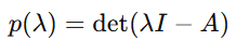
Suppose that A is a n×n matrix over a field F and that its characteristic polynomial is represented by p(𝜆)=det(λI−A), where λ is a scalar. According to the Cayley-Hamilton theorem:

This means that if you substitute the matrix A into its own characteristic polynomial, the resulting matrix expression will be the zero matrix.

Breaking it Down

1. The Characteristic Polynomial

The characteristic polynomial of matrix $A$ is defined as:

Here

• I is the identity matrix of the same size as 𝐴
• det indicates the determinant.

Example:

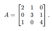
Let A be a 3×3 matrix.

The characteristic polynomial  p(λ) is defined as:

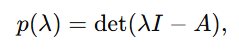
where I is the 3×3 identity matrix. Compute $\lambda I-A$:

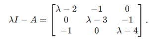
Now, compute the determinant:

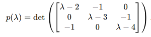
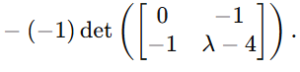
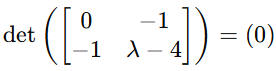
Using cofactor expansion over the first row:

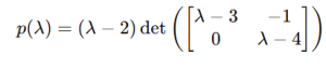
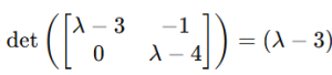
First determinant:

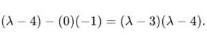
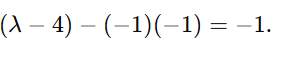
Second determinant:

Substituting back:

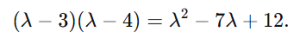
Expand (λ−3)(λ−4)

So the characteristic polynomial is:

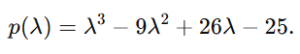
According to the Cayley-Hamilton theorem, 𝑝 ( 𝐴 ) = 0 . Replace  A with   p(λ)

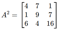
Compute A^2:

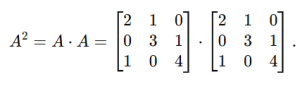
Multiply:

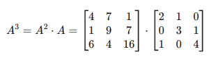
Compute A^3:

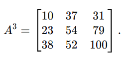
Compute p(A):

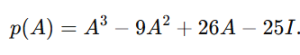
Substitute

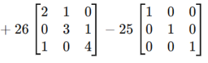
Simplify each term and add them. The result will be the zero matrix, confirming p(A)=0

Applications of the Cayley-Hamilton Theorem

1. computing the powers of a matrix.
The theorem allows us to represent higher powers of 𝐴 A using lower powers plus the identity matrix rather than multiplying it repeatedly. Polynomial relationships can simplify expressions like 𝐴 ^𝑘  for  k>n.

2. Inverse of a matrix.
The Cayley-Hamilton theorem can help identify the inverse of an invertible matrix by stating it as a sum of smaller powers of  A.

3. Differential Equations.
The Cayley-Hamilton theorem makes it easier to compute matrix exponentials in linear differential equation systems.

4. Eigenvalue analysis.
The theorem strengthens the relationship between a matrix and its eigenvalues, which are the roots of the characteristic polynomial.

The Cayley-Hamilton theorem matrix connects the abstract world of algebraic polynomials to the visible domain of matrices.