theorem
Leibnitz theorem

The proof of Leibnitz theorem is based on the concept of induction and the product rule for differentiation. This article explains how to prove the generic formula for the n-th derivative of the product of two functions.
Statement of Leibnitz Theorem:
For two differentiable functions f(x) and g(x), the n-th derivative of their product is given by:

We will prove this formula by induction.
Base case (n = 1):
For n = 1, the formula becomes the first derivative of a product:
![]()
This is exactly the standard product rule and it matches the formula with the binomial coefficient
![]() . Thus the base case holds true.
. Thus the base case holds true.
Inductive step: Assume the formula holds for some 𝑛 = 𝑘 .We assume that:

Now, we want to prove that the formula holds for n=k+1. To begin, we differentiate both sides of the inductive hypothesis (the k-th derivative of f(x) and g(x)) with respect to x.


We now apply the product rule to each term in the sum. For a given term:

This yields:

Thus the sum over all i becomes:


Now we adjust the indices of the two sums:
The first section includes the term: d^(i+1)/dx^(i+1). f(x) has a summation over i from 0 to k, but we change the index of summation from 1 to k+1. Therefore, this term becomes:

In the second part, the terms involving d^(i)/dx^(i) f (x) and d^(k-i+1)/dx^(k-i+1) g (x) simply shift to:

Finally, combining these sums yields the necessary formula: n=k+1


This completes the induction.
We have demonstrated that the formula is true for all n≥ 1 using the mathematical induction principle. Thus, it is established that the Leibnitz rule applies to the n-th derivative of a product of two functions.
Leibnitz theorem is commonly employed in calculus, particularly when differentiating products of functions numerous times. It is useful for calculating higher-order derivatives of polynomial products, trigonometric functions, and other complex functions.


Cramer’s rule 2×2 , 3×3 is a method used to solve systems of linear equations using determinants. So It applies to systems of n linear equations with n variables, assuming that the determinent of the co-efficient matrix is non zero. This rule provides precise formulas for solving a system of linear equations using determinants.
Consider this system of linear equations:
![]()
where:
- A is a square matrix (with size n×n)
- x is a column vector of unknowns x_1,x_2,…,x_ n,
- b represents a column vector of constants. b_1,b_2,…,b_n
The matrix equation can be written as:

Step-by-Step Instructions for Cramer’s rule 2×2
1. Calculate the determinant of the coefficient matrix: Check if matrix A’s determinant (det(𝐴)) is non-zero. Because if det(A) = 0, the system lacks a unique solution and cannot be solved using Cramer’s Rule.
2. Construct Matrices A_1, A_2,…, A_n: For each unknown x_i, construct a new matrix A_i by substituting the i-th column of matrix A with the column vector b. Substitute the constants from vector b for the i-th column of A to produce the i-th matrix A_i.
- is formed by replacing the first column of A with b
- A2 is created by substituting b for A’s second column.
- and so on for all columns.
3. Calculate the determinants of the modified matrix: Determine the determinant of each matrix A i, denoted as det(A_i), for each i=1, 2,…,n.
4. Solve for Each x_i: The solution for each unknown x_i is given by:

for i=1,2,…,n.
For example:
Consider this system of linear equations:

The coefficient matrix is:

The column vector b is

Step 1: Firstly, Calculate det(A)
![]()
Step 2: Create matrices A_1 and A_2.
- For x, replace the first column of A with b:

- For y, change the second column of A to b:

Step 3: Compute the determinants of A_1 and A_2
![]()
![]()
then,
Step 4: Solve for x and y:


So, lastly, the solution to the system is:

Cramer’s rule 2×2 simplifies the process of solving linear equations using determinants. However, it is computationally expensive for big systems due to the necessity to calculate numerous determinants.
Practice problems
1.

2.

3.

4.


Statement (Cauchy-Schwarz Inequality):
For any two vectors 𝑢 = ( 𝑢 _1 , 𝑢_ 2 , … , 𝑢_ 𝑛 ) and 𝑣 = ( 𝑣 _1 , 𝑣 _2 , … , 𝑣 _𝑛 ), the Cauchy-Schwarz inequality states:

with equality if and only if the vectors are linearly dependent. That is, one vector is a scalar multiple of another.
This inequality limits the magnitude of the dot product of two vectors, laying the groundwork for numerous mathematical notions such as vector angle and orthogonality.
Proof:
1. Applying the concept of quadratic forms:
The expression f(t) is defined as:

t represents a real parameter.
Expanding f(t) yields:

This simplifies to:
![]()
Where
![]()
![]()
![]()
2. Non-negativity of :
As f(t) is a sum of squares, it is always non-negative.
![]()
3. Discriminant condition:
For the quadratic equation 𝑓(𝑡)=0, the discriminant must satisfy:
![]()
Simplifying, we get:
![]()
or equivalently:
![]() Substituting the definitions of 𝑎, 𝑏, and 𝑐 yields:
Substituting the definitions of 𝑎, 𝑏, and 𝑐 yields:

4. Equality condition: Equality occurs when the discriminant Δ=0, which occurs when 𝑢_ 𝑖 and 𝑣_ 𝑖 are linearly dependent, i.e., u=kv for some scalar k.
This completes the proof of the Cauchy-Schwarz inequality.
The Cauchy inequality is a fundamental result in linear algebra and analysis. It states: For vectors u,v ∈R^n or C^n:
![]()
where
![]() is the dot product and
is the dot product and ![]() is the Euclidean norm.
is the Euclidean norm.
Example 1: Real numbers
Let u=(1, 2, 3) and v=(4, -1, 2)
- Compute ⟨u,v⟩:
![]()
- Compute ∥u∥ and ∥v∥:
![]()
![]()
- Verify the inequality:
![]()
![]()
The Cauchy-Schwarz inequality is valid when 8 ≤ 294.
Example 3: Continuous Functions
Let and on the interval . The inner product is defined as:

- Calculate ⟨f,g⟩ :

- Calculate ∥f∥ and ∥g∥.


- Verify the inequality.


Since![]() the inequality holds.
the inequality holds.
Why is Cauchy-Schwarz inequality important?
The Cauchy–Schwarz Inequality is fundamental to many mathematical and scientific disciplines. Here are some places where it plays a crucial role:
Geometry of Vectors: It allows you to compute the cosine of the angle between two vectors, which leads to the concept of orthogonality.
Linear algebra is essential for demonstrating other inequalities, such as the triangle inequality in normed spaces.
Statistics: The inequality underpins the covariance and correlation measures of random variables.
Optimization is commonly utilized in problem solving and algorithm analysis.

Finding the real roots of polynomials is one of the most difficult problems to solve, especially if modern numerical methods are not used. While the Rational Root Theorem and synthetic division can help, Descartes’ Rule of Signs provides a simple yet effective method for estimating the number of positive and negative real roots of a polynomial. In this blog, we’ll look at Descartes’ Rule of Signs and how it might aid in polynomial analysis.
What is Descartes’ Rule of Signs?
Descartes’ Rule of Signs is a mathematical principle that determines the number of positive and negative real roots of a polynomial. It works by counting sign changes in the polynomial’s coefficient sequence. Observing these sign shifts allows us to forecast the number of real roots but not their exact quantities without having to solve the polynomial directly.
The Rule Explained
The rule consists of two main parts: determining the number of positive real roots and the number of negative real roots.
1. Positive Real Roots:
To determine the number of positive real roots, use the following steps:
- Write the polynomial in standard form, with terms sorted in descending order of powers of x.
- Consider the signs of the polynomial’s coefficients.
- Count the number of sign changes between successive coefficients.
- If the coefficient sequence changes from positive to negative or negative to positive, this counts as one sign change.
- Descartes’ Rule states that the number of positive real roots is either equal to the number of sign shifts or less by an even number. This means that if there are 4 sign changes, the polynomial can have 4, 2, or 0 positive real roots
2. Negative Real Roots:
To get the number of negative real roots, use these steps:
- Replace x with −x in the polynomial.
- Write a new polynomial P(−x) and check the coefficients’ signs.
- Count the number of sign changes in the coefficient sequence of P(−x).
- As with positive real roots, the number of negative real roots will either be equal to the number of sign changes or less by an even number.
Example of Descartes’ Rule of Signs
Let’s take a polynomial and apply Descartes’ Rule of Signs:
![]()
Step 1: Determine the Number of Positive Real Roots.
The coefficients are 1, -6, 12, -18, and 9.
1,−6,12,−18,9.
Signs are as follows: +, −, +, −, +
There are four sign changes: + → − , – → + , + → − , and −→+.
According to Descartes’ Rule, the number of positive real roots is either 4, 2, or zero.
Step 2: Determine the number of negative real roots.
Substitute −𝑥 for x in the polynomial:
![]()
![]()
The coefficients of P(−x) are 1, 6, 12, 18, and 9.
The signs are all +, indicating no sign changes.
Thus, the polynomial has no negative real roots.
Interpretation of Results
Descartes’ Rule of Signs applies to the polynomial
![]()
- It has 4, 2 , or 0 positive real roots.
- It has zero negative real roots.
While Descartes’ Rule does not specify the number of roots, it does present a range of possibilities that can serve as a good starting point for further research or numerical procedures.

All formulas of circle-Concepts , Properties

How to make math fun through storytelling: Chapter 3

Types of progression (AP,GP,HP progression)

Fun math learning stories: The secret of the shadow pyramid

Math problem-solving stories: The Secret of the Shadow Pyramid

Vector properties (Definition, Examples)

Three-dimensional coordinate geometry: Formulas ,Examples

Educational math stories : Chapter 5: The infinity Chamber

Algebra puzzles and riddles for children: Chapter 4- Labyrinth of patterns

How can I make algebra fun for kids? Chapter 3- Tower of Variables


Fun math learning stories: The secret of the shadow pyramid
Math problem-solving stories: The Secret of the Shadow Pyramid
Vector properties (Definition, Examples)
Three-dimensional coordinate geometry: Formulas ,Examples
Educational math stories : Chapter 5: The infinity Chamber
Algebra puzzles and riddles for children: Chapter 4- Labyrinth of patterns
-
 algebra4 months ago
Various types of matrices
-
 algebra4 months ago
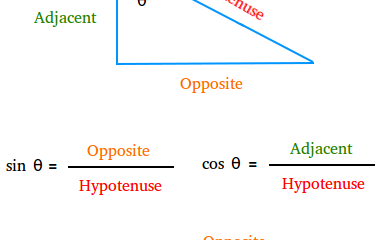
Trigonometric Rules and Formulas
-

 geometry4 months ago
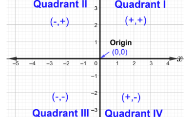
Cartesian to polar equations (Circle, line)
-

 algebra5 months ago
Different types of Matrices
-

 algebra4 months ago
Cayley-Hamilton theorem matrix
-

 algebra4 months ago
Eigenvalue of a matrix
-

 calculus5 months ago
Easy Strategies & Techniques for Effective Integration part-1
-
 geometry4 months ago
Cartesian coordinate planes (Polar to cartesian)